Getting started
Basic principles of gratopy
We start by explaining some recurring relevant quantities and concepts in gratopy, in particular the ProjectionSettings
class as well as the use of images and sinograms and the connection of forward projection to backprojection in the context of gratopy.
ProjectionSettings
The cornerstone of the gratopy toolbox is formed by the gratopy.ProjectionSettings class, which defines the considered geometry, collects all relevant
information to create the OpenCL kernels, and precomputes and saves
relevant quantities. Thus, virtually all functions of gratopy require an object of this class, usually referred to as projectionsetting.
In particular, gratopy offers the implementation for two different geometric settings, the parallel beam and the fanbeam setting.
The geometry of the parallel beam setting is mainly defined by the image_width – the physical diameter of the object in question in arbitrary units, e.g., 3 corresponding to 3cm (or m, etc.) – and the detector_width – the physical width of the detector in the same unit –, both parameters of a projectionsetting. For most standard examples for the Radon transform, these parameters coincide, i.e., the detector is exactly as wide as the diameter of the imaged object, and thus, captures all rays passing through the object.
The fanbeam setting additionally requires RE – the physical distance from the source to the center of rotation – and R – the physical distance from the source to the detector – to define the geometry, see the figures below.
Moreover, the projection requires discretization parameters, i.e., the shape of the image to project and the number of detector pixels to map to. Note that these transforms are scaling-invariant in the sense that rescaling all physical quantities by the same factor creates operators which are rescaled versions of the original ones. On the other hand, changing the number of pixels of the image or the detector leaves the physical system unchanged and simply reflects a finer/coarser discretization.
The angular range for the parallel beam setting is \([0,\pi[\), while for the fanbeam setting, it is \([0,2\pi[\).
By default, it is assumed that the given angles completely partition the angular range.
In case this is not desired, a limited-angle situation
can be considered by adapting the angles and angle_weights parameters of gratopy.ProjectionSettings, impacting, for instance, the backprojection operator.
Note also that the projections considered are rotation-invariant in the sense, that projection of a rotated image yields a sinogram which is translated in the angular dimension.
Note that the angles are measured (counterclockwise) from the positive x axis and reflect the projection-direction. The positive detector-direction is the clockwise rotation of the projection-direction by \(\frac \pi 2\).
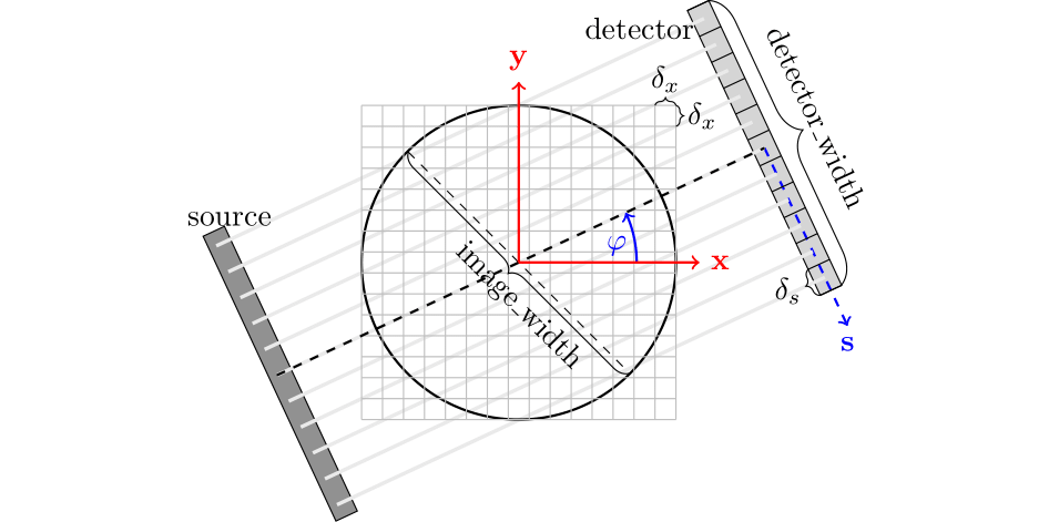
Geometry of the parallel beam setting.
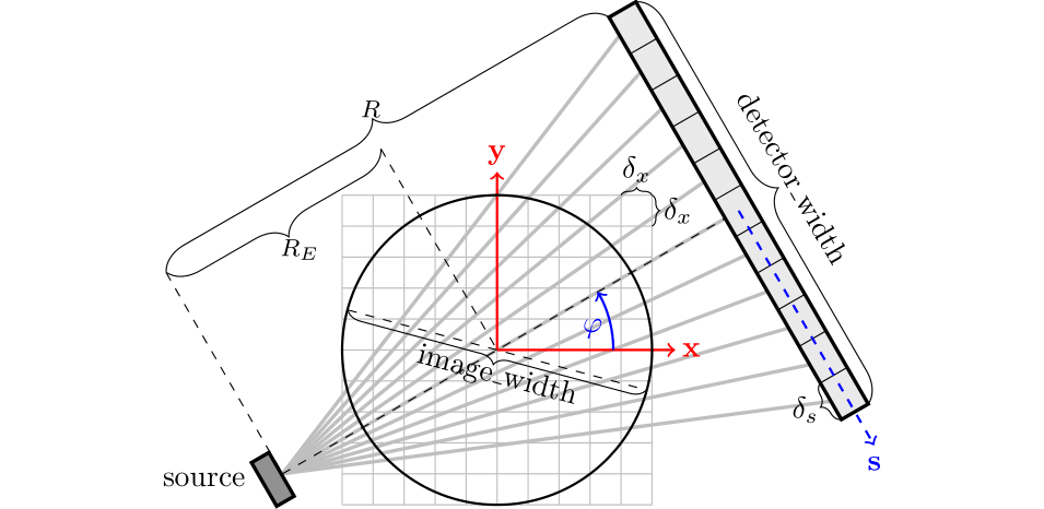
Geometry of the fanbeam setting.
The main functions of gratopy are forwardprojection and backprojection, which use a projectionsetting as the basis for computation and allow to project
an image img onto a sinogram sino and to backproject sino onto img, respectively. Next, we describe how to use and interpret images and sinograms in gratopy.
Images in gratopy
An image img is represented in gratopy by a pyopencl.array.Array of dimensions \((N_x,N_y)\)
– or \((N_x,N_y,N_z)\) for multiple slices – representing a rectangular grid of equidistant quadratic pixels of size \(\delta_x=\mathrm{image\_width}/\max\{N_x,N_y\}\),
where the associated values correspond to the average mass inside the area covered by each pixel. The area covered by the pixels is called the image domain, and the image array
can be associated with a piecewise constant function on the image domain. Usually, we think of the investigated object as being circular and contained in
the rectangular image domain. More generally, image_width corresponds to the larger side length of a rectangular \((N_x,N_y)\) grid of quadratic image pixels
which allows considering slim objects.
The image domain is, however, always a rectangle or square
that is aligned with the x and y axis.
When using an image together with projectionsetting – an instance of gratopy.ProjectionSettings – the values \((N_x,N_y)\) have to coincide with the attribute img_shape of projectionsetting, we say they need to be compatible. The data type
of this array must be numpy.float32 or numpy.float64, i.e., single or double precision, and can have either C or F contiguity.
Note that in gratopy, the first and second axis of an image array corresponds to the x and y axis, respectively, as depicted in the figures above.
Sinograms in gratopy
Similarly, a sinogram sino is represented by a pyopencl.array.Array of the shape \((N_s,N_a)\) or \((N_s,N_a,N_z)\) for \(N_s\) being the number of detectors and \(N_a\) being the number of angles for which projections are considered.
When used together with a projectionsetting of class gratopy.ProjectionSettings, these dimensions must be compatible, i.e., \((N_s,N_a)\) has to coincide with the sinogram_shape attribute of projectionsetting.
The width of the detector is given by the attribute detector_width of projectionsetting and the detector pixels are equidistantly partitioning the detector line with detector pixel width
\(\delta_s=\mathrm{detector\_width}/N_s\). The angles, on the other hand, do not need to be equidistant or even partition the entire angular range; gratopy allows for rather general angle sets. The values associated with pixels in the sinogram again correspond to the average
intensity values of a continuous sinogram counterpart and thus can be associated with a piecewise constant function. The data type of this array must be numpy.float32 or numpy.float64, i.e., single or double precision, and can have either C or F contiguity.
Adjointness in gratopy
Gratopy allows a great variety of geometric setups for the forward
projection and the backprojection. One particular feature is
that forward projection and backprojection are adjoint operators,
which is important, for instance, in the
context of optimization algorithms. Here, adjointness is achieved
with respect to natural scalar products in image and sinogram Hilbert space
that we wish to clarify in the following.
As described above, the discrete values in an image array are associated
with values of piecewise constant functions inside square pixels
(of area \(\delta_x^2\)) in the image domain.
For such piecewise constant functions, the classical \(L^2\) scalar product
is considered, which results in \(\langle \text{img1}, \text{img2} \rangle = \delta_x^2 \sum_{x,y} \text{img1}_{x,y} \text{img2}_{x,y}\)
for image arrays img1 and img2.
Similarly, the discrete values of the sinogram are associated with a piecewise
constant function on the Cartesian product of an interval of length
detector_width and the angular domain. Correspondingly, the natural inner product for the sinogram space is given by
\(\langle \text{sino1}, \text{sino2} \rangle = \delta_s \sum_{s,a} \Delta_a \text{sino1}_{s,a} \text{sino2}_{s,a}\), where \(\Delta_a\)
denotes the length of the angular range covered (in the sense of piecewise constant discretization)
by the a-th angle (by default, all \(\Delta_a\) are determined automatically based on the angles parameter, for more information on angle_weights, see gratopy.ProjectionSettings).
Hence, the implementations of the forward and backprojection in gratopy are to be understood in this
context, and in particular, the forward projection and backprojection operator are adjoint
with respect to these scalar products, as can be observed in tests.test_radon.test_adjointness() and tests.test_fanbeam.test_adjointness().
Though this is, in a sense, the natural discretization and sense of adjointness, it might be of interest to consider adjointness in a different sense. In this respect, gratopy allows to alter the sinogram space by manually setting the angle weights \((\Delta_a)_a\) to desired values, which changes the weights in the backprojection, but always leads to an adjoint operator in the sense of the aforementioned scalar products.
For example, all angles can be weighted equally with 1 in a sparse angle setting. When setting angle_weights \(\Delta_a=\frac {\delta_x^2}{\delta_s}\), the operators are adjoint with respect to the standard scalar products \(\langle \text{img1}, \text{img2} \rangle = \sum_{x,y}\text{img1}_{x,y}\text{img2}_{x,y}\) and \(\langle \text{sino1}, \text{sino2} \rangle = \sum_{s,a} \text{sino1}_{s,a}\text{sino2}_{s,a}\).
First example: Radon transform
One can start in Python via the following simple code which computes the forward and backprojection of a phantom:
# initial import
import numpy as np
import pyopencl as cl
import matplotlib.pyplot as plt
import gratopy
# discretization parameters
number_angles = 60
number_detectors = 300
Nx = 300
# Alternatively to number_angles one could give as angle input
# angles = np.linspace(0, np.pi, number_angles+1)[:-1]
# create pyopencl context
ctx = cl.create_some_context()
queue = cl.CommandQueue(ctx)
# create phantom as test image (a pyopencl.array.Array of dimensions (Nx, Nx))
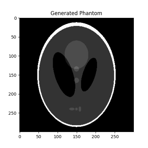
phantom = gratopy.phantom(queue,Nx)
# create suitable projectionsettings
PS = gratopy.ProjectionSettings(queue, gratopy.RADON, phantom.shape,
number_angles, number_detectors)
# compute forward projection and backprojection of created sinogram
# results are pyopencl arrays
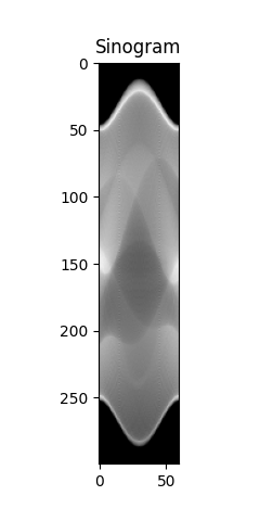
sino = gratopy.forwardprojection(phantom, PS)
backproj = gratopy.backprojection(sino, PS)
# plot results
plt.figure()
plt.title("Generated Phantom")
plt.imshow(phantom.get(), cmap="gray")
plt.figure()
plt.title("Sinogram")
plt.imshow(sino.get(), cmap="gray")
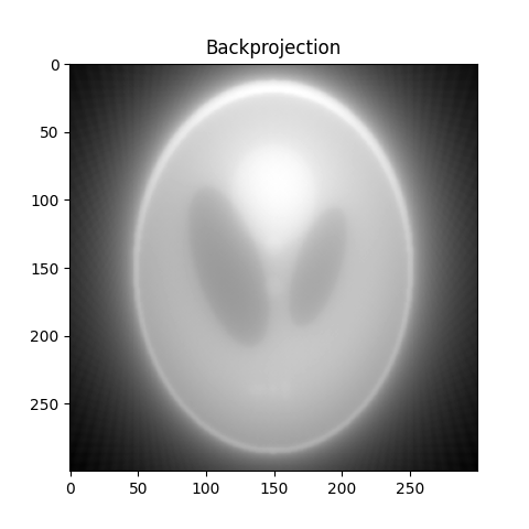
plt.figure()
plt.title("Backprojection")
plt.imshow(backproj.get(), cmap="gray")
plt.show()
The following depicts the plots created by this example.
|
|
|
Second example: Fanbeam transform
As a second example, we consider a fanbeam geometry that has a detector that is 120 (cm) wide, the distance from the the source to the center of rotation is 100 (cm),
while the distance from the source to the detector is 200 (cm). We do not choose the image_width but rather let gratopy automatically determine a suitable image_width. We visualize the defined geometry via the gratopy.ProjectionSettings.show_geometry method.
# initial import
import numpy as np
import pyopencl as cl
import matplotlib .pyplot as plt

import gratopy

# discretization parameters
number_angles = 60
number_detectors = 300
image_shape = (500, 500)

# create pyopencl context
ctx = cl.create_some_context()
queue = cl.CommandQueue(ctx)

# physical parameters
my_detector_width = 120
my_R = 200
my_RE = 100

# fanbeam setting with automatic image_width
PS1 = gratopy.ProjectionSettings(queue, gratopy.FANBEAM,
                                 img_shape=image_shape,
                                 angles=number_angles,
                                 n_detectors=number_detectors,
                                 detector_width=my_detector_width,
                                 R=my_R, RE=my_RE)


print("image_width chosen by gratopy: {:.2f}".format((PS1.image_width)))

# fanbeam setting with set image_width
my_image_width = 80.0
PS2 = gratopy.ProjectionSettings(queue, gratopy.FANBEAM,
                                 img_shape=image_shape,
                                 angles=number_angles,
                                 n_detectors=number_detectors,
                                 detector_width=my_detector_width,
                                 R=my_R, RE=my_RE,
                                 image_width=my_image_width)

# plot geometries associated to these projectionsettings
fig, (axes1, axes2) = plt.subplots(1,2)
PS1.show_geometry(np.pi/4, figure=fig, axes=axes1, show=False)
PS2.show_geometry(np.pi/4, figure=fig, axes=axes2, show=False)
axes1.set_title("Geometry chosen by gratopy as: {:.2f}".format((PS1.image_width)))
axes2.set_title("Geometry for manually-chosen image_width as: {:.2f}"
                .format((my_image_width)))
plt.show()
Once the geometry has been defined via the projectionsetting, forward and backprojections can be used just like for the Radon transform in the first example.
Note that the automatism of gratopy chooses image_width = 57.46 (cm). When looking at the corresponding plot via gratopy.ProjectionSettings.show_geometry, the image_width is such that the entirety of an object inside
the blue circle (with diameter 57.46) is exactly captured by each projection, and thus, the area represented by the image corresponds to the yellow rectangle and blue circle which is the smallest rectangle to capture the entire object. On the other hand, the outer red circle illustrates the diameter of the smallest circular object entirely containing the image.
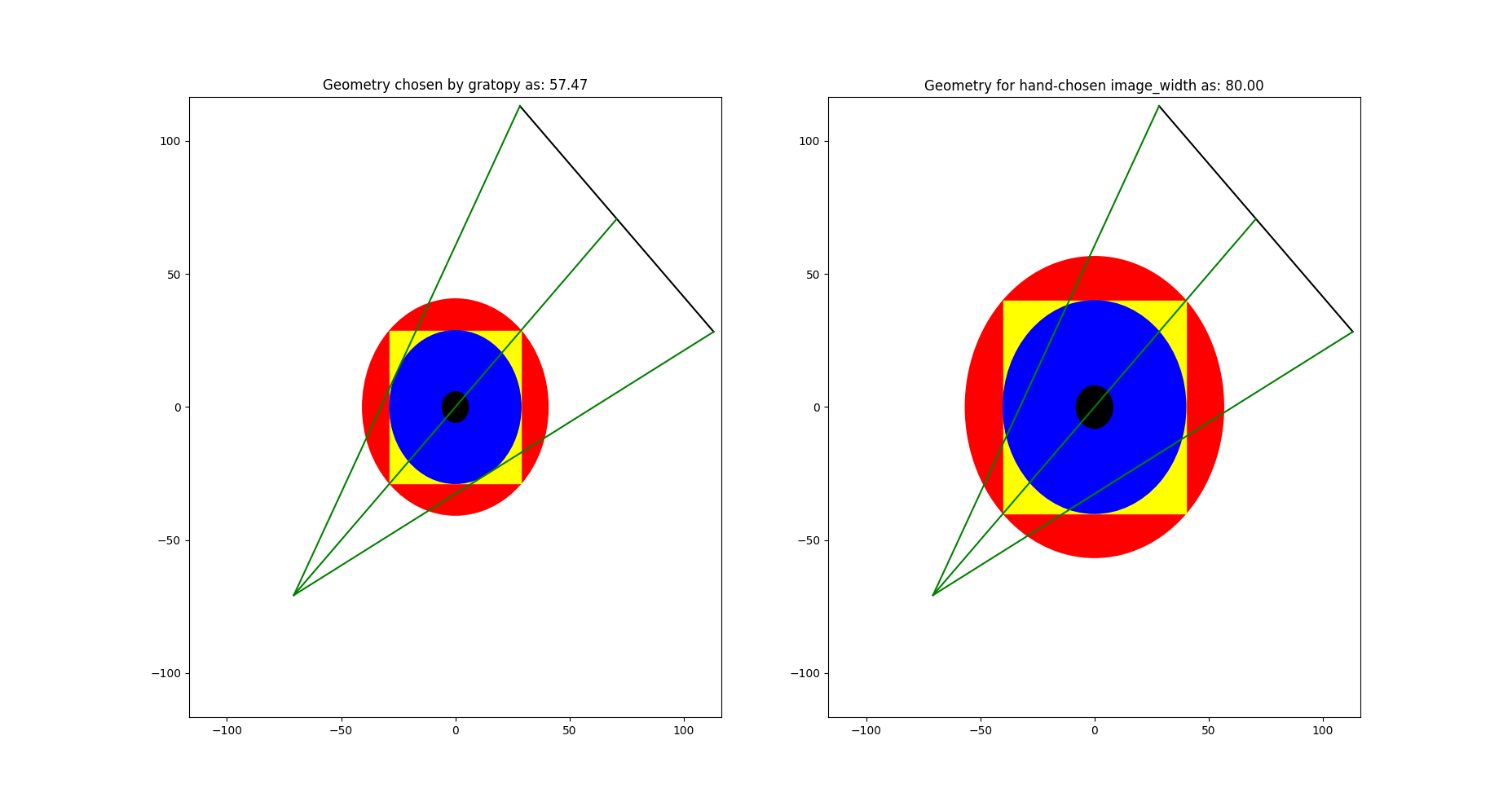
Plot produced by gratopy.ProjectionSettings.show_geometry for the fanbeam setting with automatic and manually chosen image_width, both for projection from 45°.
Further examples can be found in the source files of the Test examples.